Jupter notebook demostration¶

1. Using tab for searching (modules, attribues ...etc)
2. Auotmatic print out the last line in each ecll

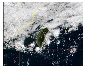
Himwari pic¶

[1]:

import cwbplot.IO_himawari_tools as tools
import  matplotlib.pyplot as plt

[2]:

out=tools.HIMAWARI('202105250000')
print(type(out))
type(out)

<class 'cwbplot.IO_himawari_tools.HIMAWARI'>

[2]:

cwbplot.IO_himawari_tools.HIMAWARI

[3]:

# show object info
#

[4]:

## get projection info of himawari
bm=out.get_basemap()
bm.imshow(out.data_rgb)

[4]:

<matplotlib.image.AxesImage at 0x7fc546b6ef28>

XML file¶

[6]:

import cwbplot.tools as tool

[8]:

## how to use
print(tool.read_xml_cwb.__doc__)

  read_xml_cwb(data_time_str,var_list,prefix='')
     data_time_str: string format(YYYYMMDDHHNN) in UTC

[9]:

## Introduce pandas format
out=tool.read_xml_cwb('202105250000','ELEV WSPD WDIR HUMD')
out

[9]:

	lat	lon	ELEV	WDIR	HUMD
466940	25.133314	121.740475	26.7	30.0	1.00
466900	25.164889	121.448906	19.0	300.0	0.82
466880	24.997647	121.442017	11.0	60.0	0.80
466930	25.162078	121.544547	607.1	200.0	0.98
466910	25.182586	121.529731	832.6	210.0	1.00
...	...	...	...	...	...
C0M800	23.299075	120.664767	440.0	0.0	0.67
C0K560	23.686450	120.603417	117.0	0.0	0.70
C0K550	23.514319	120.229736	15.0	42.0	0.73
C0X290	23.267772	120.125481	10.0	27.0	0.81
C0X310	23.147289	120.086253	9.0	19.0	0.75

529 rows × 5 columns

[10]:

out.insert(0,'yyyymmddhhnn','202105250000')
out

[10]:

	yyyymmddhhnn	lat	lon	ELEV	WDIR	HUMD
466940	202105250000	25.133314	121.740475	26.7	30.0	1.00
466900	202105250000	25.164889	121.448906	19.0	300.0	0.82
466880	202105250000	24.997647	121.442017	11.0	60.0	0.80
466930	202105250000	25.162078	121.544547	607.1	200.0	0.98
466910	202105250000	25.182586	121.529731	832.6	210.0	1.00
...	...	...	...	...	...	...
C0M800	202105250000	23.299075	120.664767	440.0	0.0	0.67
C0K560	202105250000	23.686450	120.603417	117.0	0.0	0.70
C0K550	202105250000	23.514319	120.229736	15.0	42.0	0.73
C0X290	202105250000	23.267772	120.125481	10.0	27.0	0.81
C0X310	202105250000	23.147289	120.086253	9.0	19.0	0.75

529 rows × 6 columns

[11]:

out[['lat','lon','ELEV']]

[11]:

	lat	lon	ELEV
466940	25.133314	121.740475	26.7
466900	25.164889	121.448906	19.0
466880	24.997647	121.442017	11.0
466930	25.162078	121.544547	607.1
466910	25.182586	121.529731	832.6
...	...	...	...
C0M800	23.299075	120.664767	440.0
C0K560	23.686450	120.603417	117.0
C0K550	23.514319	120.229736	15.0
C0X290	23.267772	120.125481	10.0
C0X310	23.147289	120.086253	9.0

529 rows × 3 columns

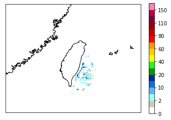
QPE file¶

[5]:

import cwbplot.IO_tools as tools

[6]:

QPE_dat='/IFS6/data2/datawrf/p108/QPESUMS/data/QPE_2D_2019012800.dat'

[7]:

out=tools.QPE_2D_READ(QPE_dat)
bm.drawcoastlines()
bm.contourf(out.lon,out.lat,out(),**out.cwbcolorbar(),latlon=True)
plt.colorbar()

[7]:

<matplotlib.colorbar.Colorbar at 0x7fc5469a1a58>

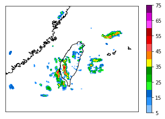
Radar CV¶

[10]:

compress_dat='/IFS6/data2/datarfs/c164/test_data/radar/COMPREF/COMPREF.20181123.0000'
compress_dat='/IFS6/data2/datarfs/c164/test_data/radar/COMPREF/CREF_030min.20210601.040000.gz'

out=tools.COMPREF_READ(compress_dat)
bm.drawcoastlines()
bm.contourf(out.lon,out.lat,out(),**out.cwbcolorbar(),latlon=True)
plt.colorbar()
print(out)

unzip files
CWB CREF binary format([('', '<i2')])
TIME:Tue Jun  1 04:00:00 2021
DIMX,DIMY,DIMZ=1501,1501,1

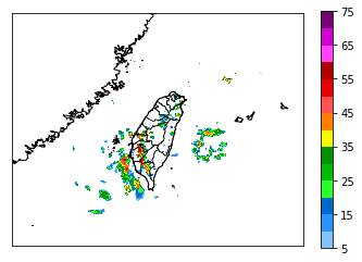
[16]:

%matplotlib inline
import cwbplot.plotwrfvar as pltwrf
import numpy as np
MREF_dat='/IFS6/data2/datarfs/c164/test_data/radar/MREF/MREF3D21L.20210601.0400.gz'
#MREF_dat='/IFS6/data2/datarfs/c164/test_data/radar/MREF/MREF3D30L.20200212.0000'

out=tools.COMPREF_READ(MREF_dat)
print(out)
print('-------colorbar')
print(out.cwbcolorbar()['levels'])

pltwrf.state(bm)
#print((out.lat))
bm.drawcoastlines()
bm.contourf(out.lon,out.lat,np.max(out(),axis=2),**out.cwbcolorbar(),latlon=True)
#bm.pcolormesh(out.lon,out.lat,np.max(out(),axis=2),vmin=5,vmax=75,cmap=out.cwbcolorbar()['cmap'],latlon=True)
plt.colorbar()

unzip files
CWB mosaicked refl binary format([('', '<i2')])
TIME:Tue Jun  1 04:00:00 2021
DIMX,DIMY,DIMZ=441,561,21

-------colorbar
[5, 10, 15, 20, 25, 30, 35, 40, 45, 50, 55, 60, 65, 70, 75]

[16]:

<matplotlib.colorbar.Colorbar at 0x7fc54440dda0>

Radar Sweep¶

[19]:

import cwbplot.cwb_radar_all as cwb_ra
from pyart.graph import RadarMapDisplayBasemap
import matplotlib.colors as mcolors
import matplotlib.pyplot as plt
import numpy as np


## You are using the Python ARM Radar Toolkit (Py-ART), an open source
## library for working with weather radar data. Py-ART is partly
## supported by the U.S. Department of Energy as part of the Atmospheric
## Radiation Measurement (ARM) Climate Research Facility, an Office of
## Science user facility.
##
## If you use this software to prepare a publication, please cite:
##
##     JJ Helmus and SM Collis, JORS 2016, doi: 10.5334/jors.119

[20]:

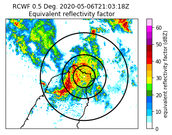
fname="/IFS6/data2/datarfs/c164/test_data/radar/RCWF.20200506.2103.bref_raw.01"
radar = cwb_ra.read_cwb_radar_sweep(fname)
display1 = RadarMapDisplayBasemap(radar)
cwb_data=['None','#9BFFFF','#00CFFF','#0198FF','#0165FF','#309901','#32FF00','#F8FF00','#FFCB00','#FF9A00','#FA0300','#CC0003','#A00000','#98009A','#C304CC','#F805F3','#FECBFF']
cmap = mcolors.ListedColormap(cwb_data,'precipitation')
norm = mcolors.BoundaryNorm(list(range(0,66,5)), cmap.N)
display1.plot_ppi_map(list(radar.fields.keys())[0], sweep=0, resolution='h',
                         vmin=0, vmax=65, min_lon=120, max_lon=123,
                         min_lat=24, max_lat=26.25,cmap = cmap,
                         mask_outside=True,
                         projection='aeqd')

display1.plot_range_rings([25,50,100])

/home/c052/Pub/anaconda3/envs/plotenv/lib/python3.6/site-packages/pyart/graph/radarmapdisplay_basemap.py:81: DeprecationWarning: RadarMapDisplayBasemap is deprecated in favor of RadarMapDisplay. Basemap is still optional to use, but there will be no support if an error appears.
  DeprecationWarning)

[Bonus] The possibility of plot manipulation¶

[21]:

import cwbplot.plotwrfvar as pltwrf
import cwbplot.IO_tools as IO
from mpl_toolkits.basemap import Basemap
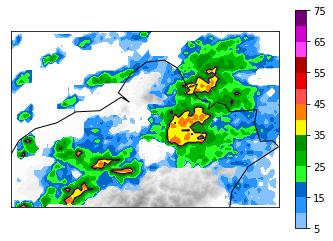
compress_dir='/IFS6/data2/datarfs/c164/test_data/radar/COMPREF/COMPREF.20181123.0000'

[22]:

%matplotlib inline
out=IO.COMPREF_READ(compress_dir)
bm = Basemap(resolution='i',rsphere=(6370000.00,6370000.00),projection='lcc', llcrnrlon=121, urcrnrlon=122, llcrnrlat=24.8, urcrnrlat=25.4,lat_1 = 10., lat_2 = 40.,lon_0 = 121.76013, lat_0 = 24.128498)
pltwrf.terrain(bm,cmap='binary')
bm.contourf(out.lon,out.lat,out(),**out.cwbcolorbar(),latlon=True)
plt.colorbar()
CS=bm.contour(out.lon,out.lat,out(),[35],latlon=True)

bm.drawcoastlines()

[22]:

<matplotlib.collections.LineCollection at 0x7fcae09a36a0>

[23]:

from shapely.geometry import Polygon
poly_list=list()
for i in range(len(CS.collections[0].get_paths())):

    p = CS.collections[0].get_paths()[i]
    v = p.vertices
    x = v[:,0]
    y = v[:,1]
    try:
        poly = Polygon([(i[0], i[1]) for i in zip(x,y)])
        poly_list.append(poly)
    except:
         pass

[24]:

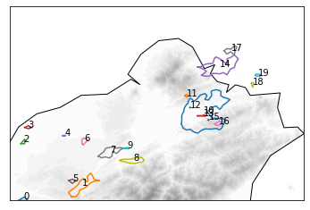
fig,ax = plt.subplots()
bm = Basemap(resolution='i',projection='cyl', llcrnrlon=121, urcrnrlon=122, llcrnrlat=24.9, urcrnrlat=25.3)

bm = Basemap(resolution='i',rsphere=(6370000.00,6370000.00),projection='lcc', llcrnrlon=121, urcrnrlon=122, llcrnrlat=24.8, urcrnrlat=25.4,lat_1 = 10., lat_2 = 40.,lon_0 = 121.76013, lat_0 = 24.128498)

pltwrf.terrain(bm,cmap='binary')
for i in range(len(poly_list)):
    x,y=poly_list[i].exterior.xy
    aa=poly_list[i].centroid.coords[0]
    plt.annotate(str(i),xy=(aa))
    ax.plot(x,y)
bm.drawcoastlines()

[24]:

<matplotlib.collections.LineCollection at 0x7fcae1487da0>

[25]:

poly_list.sort(key=lambda x:x.area,reverse=True)
for i in range(4):
    display(poly_list[i])

[14]:

from IPython.display import HTML
HTML('<iframe src="https://drive.google.com/file/d/1M_P8ZfN6rv6txj1IT4d4RXWEezmSoPq-/preview" width="640" height="480" allow="autoplay"></iframe>')

[14]:

[ ]: